Introduction
Most economists agree there are times when government borrowing is either necessary or unavoidable, such as wars and recessions. But there is less agreement on how the national debt affects the economy and whether it imposes a disproportionate burden on current or future generations.
When the government pays for itself by borrowing money instead of raising taxes, critics claim the burden is shifted from current taxpayers to future taxpayers. According to this view, the national debt necessitates a future tax increase on our children and grandchildren. But some economists say raising taxes to repay the national debt doesn’t burden future generations because “we owe it to ourselves.”[1] This argument ignores the distinction between those who lend money to the government and those who repay the debt with higher taxes.
Other economists suggest that if the economy grows fast enough and interest rates are low enough, the national debt doesn’t have to be repaid. The debt can be refinanced (or rolled over) indefinitely. But this approach imposes its own burden by reducing other savings and investment, and it increases the risk of inflation or financial crisis.[2]
This issue brief will consider why the national debt matters; examine the conditions under which the national debt may not need to be repaid; and use a few basic economic models to illustrate how the national debt can redistribute income both within each generation and between different generations. The results depend on economic growth rates, interest rates, the amount of debt, and who holds it. The models suggest that government borrowing primarily benefits current generations at the expense of future generations.
Why the National Debt Matters
The justification for government borrowing is often presented in terms of wars and recessions.[3] During times of war, the government borrows money to support the military. The additional debt is justified on the grounds that future generations will benefit from winning the war; therefore, they should share the burden by paying the additional taxes needed to repay the debt.[4]
During a recession workers who lose their jobs pay less taxes and collect more unemployment benefits, which means higher deficits. In addition, the government typically enacts temporary tax cuts and spending increases to stimulate the economy.[5] The additional debt is justified on the grounds that it is unavoidable due to the recession and necessary to expedite an economic recovery.[6]
These justifications implicitly acknowledge that raising taxes during a war or recession would be too burdensome and should be deferred until the war ends or the economy recovers. To the extent taxes are uniquely burdensome on the economy, the decision to issue debt now and raise taxes later shifts the burden from the present to the future.[7] But the more conventional view is that the burden of the national debt is due to its negative effect on savings and investment.
Economists often suggest when the economy is in a recession, government borrowing merely puts idle resources to use until the economy recovers.[8] But when the economy is “fully employed,” government borrowing reduces the amount of credit available to other borrowers and results in higher interest rates, thereby “crowding out” other savings and investment. As a result, future generations will have a smaller stock of capital assets (buildings, equipment, intellectual property, and inventories) and a lower standard of living. According to this view, the effect of government borrowing depends on the state of the economy.[9]
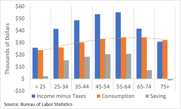
An alternative view is that the crowding out effect of government borrowing depends on how the national debt affects individual net wealth, instead of the state of the economy. This view is consistent with the life cycle-permanent income (LC-PI) hypothesis, which holds that individuals want to maintain a constant level of consumption based on their expected average lifetime income. To achieve this goal, they borrow when they are young adults to attend college, buy a home, or start a business; they pay off student loans, repay mortgages and save for retirement when they are middle-age; and they spend down their accumulated wealth when they are old. This basic pattern can be observed in Figure 1, which shows average per capita after-tax income, consumption, and savings for each age group.[10]
Figure 1: Average Per Capita After-Tax Income, Consumption and Savings by Age (2019)
Assuming most individuals behave in a manner consistent with LC-PI hypothesis, the publicly held portion of the national debt can affect their net wealth. The national debt is an asset to individuals who purchase government securities and a liability to taxpayers. If individuals repay their share of the national debt with higher taxes during their lifetime, then the effect of the national debt on net wealth is negligible because the asset is offset by the liability. If individuals redeem their share of the debt, consume the income, and die before their taxes go up and the debt is repaid, then the effect of the national debt on net wealth is significant because the asset exceeds the liability. To the extent individuals accumulate wealth to maintain consumption in retirement, an increase in the national debt will crowd out other savings and investment (see Appendix).
The Interest Rate-Growth Rate Differential
The effect of the national debt on individual net wealth depends primarily on whether the debt is repaid. Projections of rising federal budget deficits and a growing national debt suggest higher taxes will be needed to repay the debt, or at least pay the interest to avoid compounding the cost. Under certain conditions, however, the government can refinance (or roll over) the debt and neither principal nor interest would ever need to be (re)paid. The primary factors that determine whether the national debt is sustainable or not is the difference between the interest rate (r) on government securities and the growth rate of the economy (g), and whether the annual deficit excluding interest (i.e., the “primary deficit”) is equal to zero.
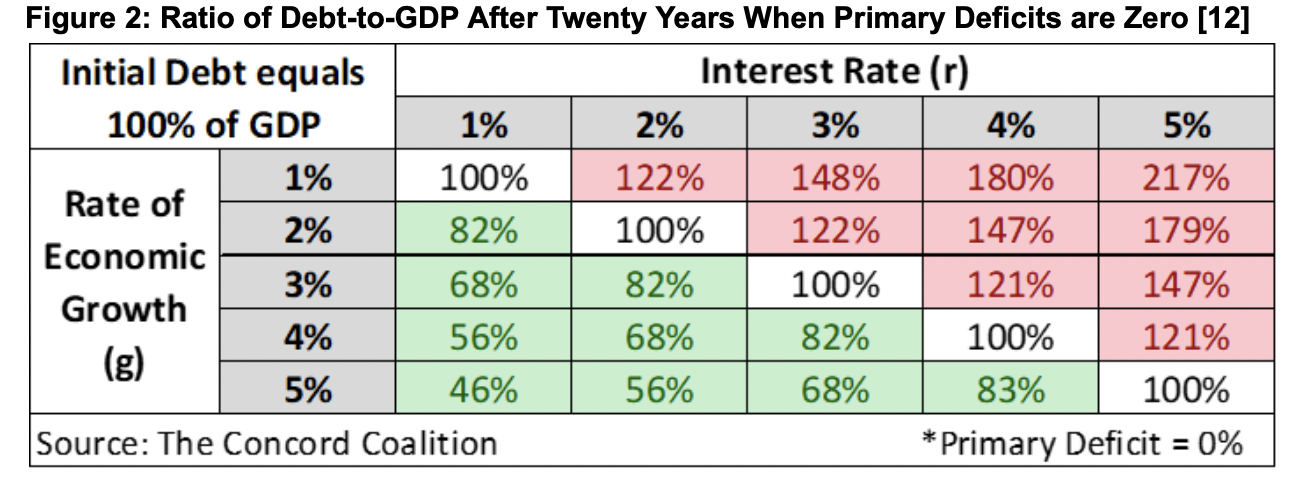
When interest rates are lower (or higher) than the rate of economic growth, then the national debt will decrease (or increase) relative to the size of the economy, as measured by Gross Domestic Product (GDP). When the rates are equal, the ratio remains constant, assuming the primary deficit is equal to zero. Figure 2 is a stylized example that shows how the debt-to-GDP ratio (starting at 100%) would either increase (r>g), decrease (r<g), or stay the same (r=g) over a twenty-year period.
But assuming primary deficits are zero (0%) is overly optimistic given our aging population and rising healthcare costs. The Congressional Budget Office (CBO) projects primary deficits will range between 2% and 5% of GDP over the next thirty years.[11] Every percentage point of primary deficits increases the interest rate-growth rate differential needed to stabilize the debt-to-GDP ratio by an additional percentage point.
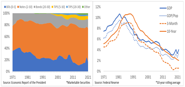
The interest rate–growth rate differential plays a critical role in determining whether the national debt will rise or fall relative to the size of the economy. Of course, the government has more than one interest rate because it issues several different types of securities (bills, notes, and bonds) with a range of maturities (0-to-1 year, 2-to-10 years, 20-to-30 years).[13] Securities with longer maturities typically pay higher interest rates than securities with shorter maturities. Thus, the weighted average interest rate on the national debt depends on the distribution of securities issued by the government.
The left side of Figure 3 shows the distribution of securities, and the right side shows the average nominal economic growth rate (both total GDP and per capita GDP) and the average nominal interest rate on 3-month and 10-year securities.[14] History provides no definitive guidance to determine the magnitude and direction of the future interest rate-growth rate differential. It has been both positive and negative in the past.[15]
Figure 3: Distribution of Securities* and Average Economic Growth and Interest Rates*
Benefits and Burdens
The benefits and burdens of the national debt can be analyzed from two different perspectives: (1) the change in income (or consumption) when the debt is incurred, and (2) the change in income (or consumption) when the debt is either repaid or rolled over. Each perspective can be illustrated with an overlapping generations (OLG) model. A neoclassical growth model can be used to illustrate the additional economic effects of crowding out.
The OLG model provides a stylized representation of the economy in which individuals work and accumulate wealth for one or more periods, and then retire and spend their wealth before dying at the end of their final period. Each generation (or birth cohort) coexists with one or more subsequent generation(s), allowing the transfer of wealth between generations.
Figure 4 shows a three-period OLG model in which each birth cohort works and saves for two periods (ages 25-44 and 45-64) and then retires and dissaves for one period (ages 65-84).[16] Assuming each cohort earns $100 each period, the combined income for all cohorts in each period is $300 (add the vertical columns) and the cumulative lifetime income for each cohort is $300 (add the horizontal rows).
Given these assumptions, if the government borrows $9 in Period 4 (equivalent to 3 percent of GDP in this example), and then raises taxes $9 to repay the debt in Period 7, total income in each period is unchanged, but lifetime income rises to $303 for cohorts B, C, and D, and falls to $297 for cohorts E, F, and G.
Figure 4: OLG Model: Debt Issuance in Period 4 and Debt Repayment in Period 7
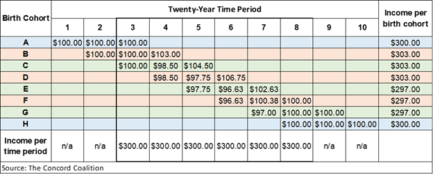
This result assumes each cohort in Period 4 lends the government $3, and the government pays each cohort in Period 4 a $3 lump-sum transfer (or rebate). Likewise, the government raises taxes on each cohort in Period 7 by $3 and repays the debt held by each cohort, which is equal to $9. This example also assumes the inflation rate, interest rate and economic growth rate are all equal to zero. Although this series of transactions might seem to have no net effect (Debt = Transfers = Taxes), that is not the case.
Assuming each cohort (B, C, and D) that incurred the debt in Period 4 sells their bonds before they die to the two younger cohorts in the corresponding period (4, 5, and 6), their lifetime income will rise by $3. On the other hand, in Period 7 when each cohort (E, F, and G) pays $3 in taxes to repay the debt, their lifetime income falls by $3. The net effect on each cohort’s income in period 7 varies due to the unequal distribution of debt resulting from the timing of the previous purchases.
This example illustrates how an increase in the national debt can benefit current generations at the expense of future generations, even without considering the additional economic effects of crowding out. Moreover, it shows why raising taxes to repay the debt does not eliminate the burden, even though “we owe it to ourselves.”
Assuming the government does not raise taxes to repay the debt, the OLG model shows continuously rolling over the debt would ultimately have no effect on lifetime income. But rolling over the debt would reduce period income by $6 when cohorts are younger, and increase period income by $6 when cohorts are older. In the context of the LC-PI hypothesis, this income shift would cause younger cohorts to either reduce their other savings or retire earlier to equalize lifetime consumption (see Appendix).
When the national debt is continuously rolled over and never repaid, the outstanding government securities become part of the net wealth of the individuals who hold them. Assuming desired wealth is the amount needed to maintain constant lifetime consumption, individuals can achieve this goal by allocating their investment portfolio between government securities and the stock of capital assets. Although the exact allocation depends on the relative rates of return, a larger national debt inevitably means a smaller capital stock upon which future economic growth depends.
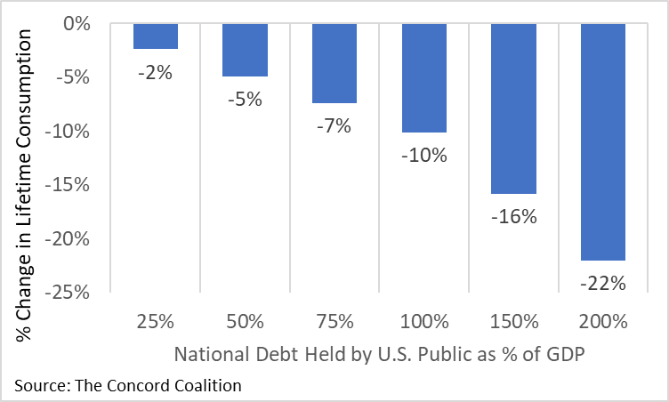
The economic effects of less capital can be estimated with a neoclassical growth model where the output of goods and services is determined by the input of labor and capital. The results of the model as shown in Figure 5 suggest every ten percentage point increase in the publicly held portion of the national debt as a share of GDP reduces the lifetime consumption of future generations by about one percent (see Appendix).
Figure 5: Economic Effects of National Debt Held by U.S. Public as a Percentage of GDP
Conclusion
The national debt may appear to shift the burden of government from the present to the future because current generations voluntarily buy government securities, whereas future generations are forced to repay the debt with higher taxes. But the burden is not defined by the voluntary or compulsory nature of the transaction, nor is it limited to the initial borrowing and subsequent repayment.
All government spending diverts resources from other uses and imposes a cost in terms of forgone alternatives. This opportunity cost exists regardless of the means of finance – raising taxes, issuing debt, or printing money. Although the means of finance does not affect the value of government spending, which ranges from useful to wasteful, it does affect who benefits and who bears the burden of paying for the spending. Ultimately, the national debt primarily benefits current generations at the expense of future generations.
* * *
Appendix – Economic Effects of a Permanent National Debt in a LC-PI Growth Model
To the extent individuals anticipate a lack of future income due to illness, unemployment, or retirement, they will save a portion of their current income. In the absence of government taxes and transfers, the amount they need to save depends on the rate of return on investment (roi), the rate of economic growth (g), and their desired savings goal. Note (roi) refers to the rate of return on the stock of capital assets, which differs from (r) discussed previously in the issue brief, which refers to the rate of return on government securities.
The life cycle-permanent income (LC-PI) hypothesis holds that individuals want to maintain a constant level of consumption based on their expected average lifetime income. Assuming individuals work from ages 25 to 64 and retire from ages 65 to 84, and both (roi) and (g) are equal to zero, they would need to save one-third of their annual wages to maintain constant consumption (see left side of Figure A1). Additional savings would be needed to cover the loss of wages due to disability or unemployment prior to retirement.
Figure A1: Savings and Consumption with and without Taxes and Transfers by Age
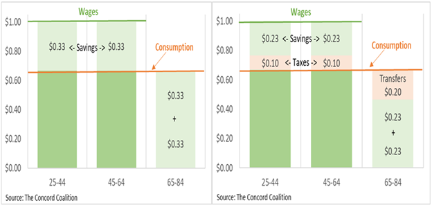
Government taxes and transfer programs like Social Security, Medicare, and Unemployment Insurance reduce the amount of savings needed by providing an alternative source of income to individuals who are not working. Individuals pay taxes in addition to saving a portion of their wages and collect transfer payments in addition to drawing down their savings (see right side of Figure A1).
Taxes and transfers do not necessarily reduce savings by an equal amount. The size of the offset depends on whether individuals view taxes and transfers as a substitute or supplement to savings. Workers could use transfers to substitute for a portion of their savings and retire at the same age, or they could use transfers to supplement their savings and retire at an earlier age. Workers retiring at an earlier age need more savings (or larger transfers) to support themselves during their additional years in retirement (Figure A2).
Figure A2: Taxes and Transfers Can Offset Savings and/or Reduce Retirement Age

The effect of government taxes and spending on savings and investment is further complicated when the spending is financed by borrowing, instead of taxes. Admittedly, the national debt is equal to the present value of the future taxes needed to repay the debt.[17] But the national debt is an asset to debtholders and a liability to taxpayers. Unless debt, taxes, and transfers are purchased, paid, and received in equal and offsetting amounts by the same individuals, the national debt cannot be neutral with respect to savings and investment.
The government primarily borrows from individuals indirectly through financial intermediaries like banks, insurance companies, and pension funds. The government securities held by these intermediaries add to the net wealth of individuals to the extent the present value of the securities exceeds the present value of the taxes needed to repay them. If individuals sell their securities, consume the proceeds, and die before taxes go up to repay them, they will receive the full value of the securities, in addition to any other government transfers they received that were financed with the initial borrowing.
Depending on when the government borrows, how it spends the money, and when it raises taxes to repay the debt, or rolls it over, the net effect will be to redistribute income within generations, between generations, or both. These results can be illustrated with an overlapping generations (OLG) model.
The OLG model provides a stylized representation of the economy in which individuals work and accumulate wealth for one or more periods, and then retire and spend down their wealth before dying at the end of their final period. Each generation (or birth cohort) coexists with one or more subsequent generation(s), allowing the transfer of wealth between generations.
To focus on the effects of borrowing and repayment or rolling over debt – instead of the effects of progressive taxes and redistributive transfers – the model assumes the government borrows an equal amount from each cohort in one or more periods, spends the money on equal lump-sum transfers (or rebates) to each cohort in the corresponding period or periods, and repays the debt with lump-sum taxes on each cohort in a subsequent period; or in some scenarios the debt is rolled over and never repaid.
As previously shown in Figure 4 of the issue brief, the OLG model illustrates how borrowing and repayment can increase the lifetime income of some cohorts when the debt is incurred and decrease the lifetime income of subsequent cohorts when the debt is repaid. These results vary slightly depending on whether the interest rate (r) is greater than, less than, or equal to the rate of economic growth (g) as shown on the left side of Figure A3 below.
Figure A3: Lifetime Income by Birth Cohort with and without Debt Repayment
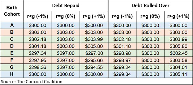
Alternatively, the government might choose to roll over the debt without ever repaying it. In that scenario, the results again vary slightly depending on the values of (r) and (g). Following the initial increase in the lifetime income of cohorts living in the period when the debt is incurred, the lifetime income of subsequent cohorts either increases (r>g), stays the same (r=g), or decreases (r<g), as shown in the right side of Figure A3.
When r>g, the government would incur additional debt to pay interest on the initial debt. This result creates a Ponzi scheme in which each generation enjoys a higher lifetime income by selling their government securities to subsequent generations. But rising levels of debt can produce rising lifetime incomes only if subsequent cohorts are willing to devote an increasingly larger share of their annual income to purchasing government securities from preceding cohorts. This result is unsustainable because it violates the LC-PI hypothesis.
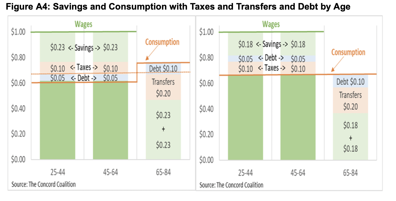
If workers buy government securities from retirees by reducing current consumption, they will increase future consumption in retirement (left side of Figure A4). To equalize lifetime consumption, individuals would have to retire before age 65. But that would reduce the supply of labor, which would reduce the output of goods and services. Alternatively, if workers buy government securities from retirees by reducing current savings, they will maintain constant lifetime consumption (right side of Figure A4). But less savings will result in less investment in the stock of capital assets, which will reduce the output of goods and services.
To determine the effect of a permanent national debt on the overall economy, it’s necessary to consider the accumulation and transfer of wealth between generations in the context of the LC-PI hypothesis combined with a neoclassical growth model where the output of goods and services is determined by the input of labor and capital.[18]
As shown in Figure A5, the value (replacement cost) of the stock of capital assets (buildings, equipment, intellectual property, and inventories) for the entire economy (businesses, households, and government) has averaged nearly three times the amount of income derived from the output of goods and services, and income has been split roughly 60/40 between labor and capital, respectively.[19]
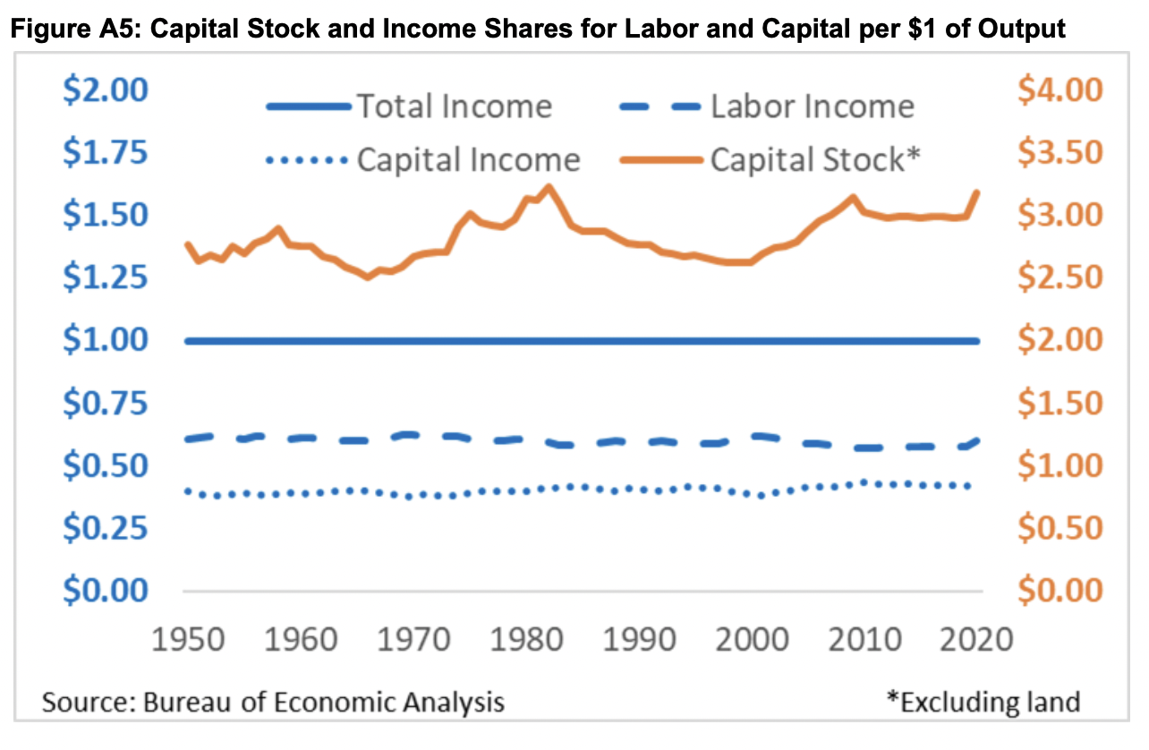
These historical relationships are used to calibrate the neoclassical growth model and determine how much individuals work, save, and invest, and when they retire, under alternative assumptions about the size of the national debt relative to the size of the economy.
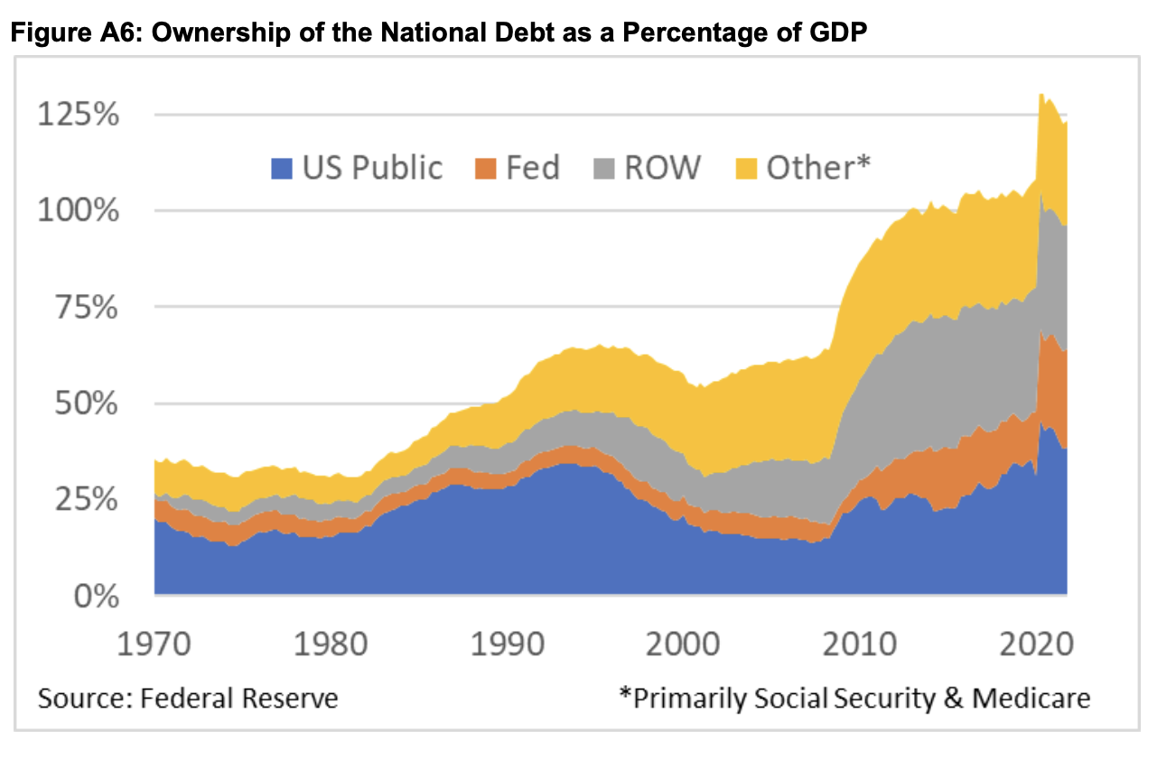
This analysis focuses on the share of the national debt held by the U.S. public, instead of the shares held by the Federal Reserve (Fed), government trust funds (Other), and the rest of the world (ROW).[20] Debt held by the Fed is used to conduct monetary policy and does not add to net wealth. Debt held by government trust funds like Social Security and Medicare do add to net wealth because individuals are entitled to defined benefits, not trust fund bonds. Including both benefits and bonds is double counting. If the government ultimately borrows from the public to redeem trust fund bonds, then the additional government securities would add to net wealth as long as publicly held debt is not repaid by raising taxes on those who hold it. Debt held by ROW is discussed below.
In the context of the LC-PI hypothesis, the amount of crowding out depends on how much the rate of return on investment (roi) in the capital stock exceeds the interest rate (r) on government securities. As Figures A1 and A4 show, individuals must forgo consumption when working to maintain consumption in retirement. Every $1 of investment reduces current consumption by $1, regardless of whether individuals invest in the capital stock or buy government securities. But $1 of capital provides more future consumption than $1 of securities because the return on capital is higher than the return on securities. Thus, to equalize lifetime consumption, workers must adjust consumption, investment allocation (capital stock vs government securities), and retirement age to account for the difference between (roi) and (r).
The rate at which individuals are willing to forgo current consumption in exchange for future consumption is the rate of time preference. This rate can be used to convert present values into future values or vice versa. Assuming (g) and (r) are equal to zero and the model is calibrated to the values shown in Figure A5, the (roi) equals 2.0% when calculated as an internal rate of return on a fixed lifetime annuity. Given this return differential, workers who invest $1 in the capital stock at age 25 would be able to consume $2.21 at age 65 ($1*1.02^40), whereas workers who invest $1 in government securities would be able to consume $1 at age 65 ($1*1.00^40).
While the concept of time preference is usually expressed in terms of forgoing $1 in the present in exchange for $2.21 in the future, the concept can also be expressed in terms of converting future values into present values. Thus, $2.21 of future consumption would have a discounted present value of $1 ($2.21/1.02^40), whereas $1 of future consumption would have a discounted present value of $0.45 ($1/1.02^40).

As shown in Figure A7, when workers invest $1 in government securities instead of the capital stock, they forgo $0.55 in future consumption ($1.00-$0.45), when measured on a discounted present value (DPV) basis. This differential can be used to calculate the amount of crowding out that occurs in the model. When the number of working years (40) is twice the number of retirement years (20), for example, crowding out is the value of (x) that equalizes lifetime consumption: 40/60-D*(1-x) = 2*(20/60-D*x)+2*D/1.02^40, which simplifies to x = (2/1.02^40+1)/3. Although the debt (D) variable cancels out of the equation, the amount of debt affects the return differential (roi – r) as explained below.
Figure A8 shows if workers reduced their capital investment to purchase government securities, they would consume $0.67 while working and $0.61 in retirement (Crowding Out = 100%). If they reduced their consumption to purchase government securities, they would consume $0.62 while working and $0.71 in retirement (Crowding Out = 0%). If they reduced both consumption and capital investment based on the return differential, they would consume $0.65 while working and $0.65 in retirement.

The amount of crowding out derived from the LC-PI hypothesis can be combined with the neoclassical growth model to determine the economic effects of increasing the national debt. The model is calibrated to the average historical values (Figure A5) to establish an initial baseline scenario. When the national debt is increased by specified amounts, the model adjusts consumption, investment, employment, and retirement to restore constant lifetime consumption under each of the alternative scenarios.
The baseline scenario assumes (g) and (r) are equal to zero, (roi) is equal to 2.0%, and there is no national debt. Individuals are employed from ages 25 to 64 and then retire from ages 65 to 84. Workers invest a portion of their annual wages to accumulate ownership of the capital stock until they retire and begin to gradually sell their share of the capital stock to younger workers, allowing the transfer of ownership between generations. Workers pay more in taxes than they receive in transfers, while retirees do the reverse, resulting in a net government transfer from workers to retirees.
Under the alternative scenarios, the share of the publicly held national debt varies from 25% to 200% of GDP. (Note the publicly held share averaged 23% from 1970 through 2021 as shown in Figure A6.) The amount of debt is assumed to remain constant under each scenario when measured as a share of the baseline GDP. This assumption means debt is rising as a share of the GDP in each scenario because the alternative GDP is smaller than the baseline GDP due to the crowding out of the capital stock. This result is partially offset by the fact that a decrease (or increase) in the capital stock will increase (or decrease) the return to capital (roi) due to the law of diminishing returns. When (roi) increases relative to (r), the amount of crowding out is reduced.[21]
To the extent individuals buy government securities instead of investing in the capital stock, their annual income and lifetime consumption are reduced relative to what they would have otherwise been. Figure 5 in the issue brief shows the change in lifetime consumption for each cohort under alternative assumptions about the amount of publicly held national debt. On average, every ten percentage point increase in debt, relative to the baseline GDP, reduces lifetime consumption by about one percent.
These economic effects are potentially understated because the model assumes total factor productivity (TFP) is constant. TFP is a statistical residual that reflects the change in output that cannot be attributed to the change in inputs. Because the quality and quantity of labor and capital are difficult to measure, TFP is often attributed to an exogenous rate of technological progress unrelated to the accumulation and improvement of labor and capital. But to the extent technology is endogenous to labor and capital, less investment would reduce TFP and the negative effects of crowding out would be even more severe.
The Rest of the World
The analysis above focuses on the share of the national debt held by the US public. But the share held by the rest of the world (ROW) has been rising in recent decades (Figure A6). To understand how foreign holdings of the national debt affect the US economy, it’s necessary to review some basic economic accounting.
The US economy can be measured in two ways: (1) sources of income, and (2) uses of income. In a “closed” economy with no international trade or investment, sources of income include the amount earned by labor (L) and capital (K) from producing goods and services; and uses of income include the amount of expenditures on goods and services which are categorized as either consumption (C) or investment (I). The amount earned equals the amount spent: Income (L+K) = Expenditures (C+I).
In an “open” economy with international trade and investment, the accounting identity becomes L+K = C+I+X-M, where X is exports and M is imports.[22] Exports increase income because labor and capital earn money when US goods and services are sold to the rest of the world. But imports do not actually reduce income because C, I, and X already include imports, either as finished products or components parts. M is subtracted from the other categories (C+I+X) to avoid double counting.[23]
Historically, the allocation of expenditures between consumption and investment has been roughly constant, averaging 78% and 22%, respectively (left side of Figure A9). But expenditures have consistently exceeded income in recent decades (right side of Figure A9). These extra expenditures are possible because the US borrows from the rest of the world. This borrowing is possible because the rest of the world uses some of the dollars earned from selling their products to the US to buy US assets (capital stock and government securities), instead of US goods and services.
Figure A9: Consumption vs. Investment and the Current-Account Balance
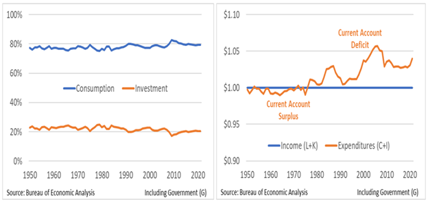
The net flow of international transactions (both trade and investment) between the US and the ROW is measured by the current-account balance, which primarily reflects the level of net exports (X-M), but also includes net international investment income, and net international transfers like gifts, pensions, and foreign aid. From 1950 through 1975, the US generally had a current-account surplus. From 1976 through 2021, the US generally had a current-account deficit.
The current-account balance can affect the US economy by changing the allocation of net wealth in the ROW (capital stock vs. government securities), and by changing the composition of expenditures in the US (consumption vs. investment).
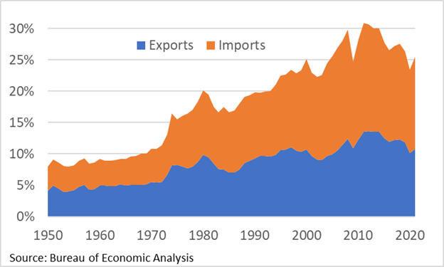
From the ROW’s perspective, buying US government securities adds to net wealth. Unlike US taxpayers, foreign investors will not be subject to the higher US taxes needed to repay the US national debt. When the ROW (excluding central banks) buys US government securities instead of investing in the capital stock, the output of goods and services will be reduced. A smaller ROW economy results in a smaller US economy because the ROW will have less income to buy US goods and services, and less ability to provide inputs needed to produce US goods and services.[24] International trade has become increasingly important to the US economy in recent decades (Figure A10).
Figure A10: U.S. Exports and Imports as a Percentage of GDP
When the ROW buys US assets, they expect to earn future income in the form of interest, dividends, capital gains, or repayment of principal. The ability of the US to make these payments to the ROW – without borrowing more from the ROW – will eventually require the US to reverse the current-account balance. To the extent current generations have been able to consume more than their income by running a current-account deficit, future generations will have to consume less than their income by running a current-account surplus. Exactly which generations will be affected depends on when the balance shifts from deficit to surplus.
In theory, the US might be able to continue borrowing from the ROW indefinitely. But eventually most (or even all) of the subsequent borrowing will be needed just to repay the previous borrowing, instead of being available to buy foreign goods and services. Thus, unlike current generations who have enjoyed an extended period of excess consumption, future generations will not have the same opportunity.
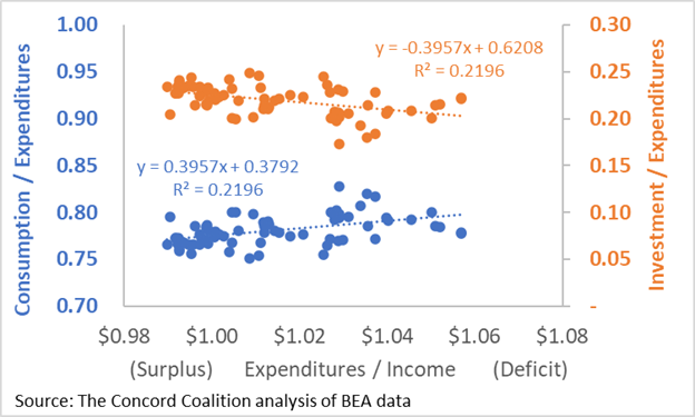
Government borrowing from the ROW also appears to affect the composition of expenditures in the US between consumption and investment. Regression analysis suggests every one percentage point increase in the current-account deficit reduces the investment share of expenditures by about one-tenth of a percentage point over the long-term.[25] This result may not reflect a permanent (or equilibrium) effect. But to the extent money borrowed from the ROW is used to fund consumption instead of investment, future generations will have less capital and lower incomes, relative to what they would have otherwise been.
Figure A11 shows the correlation between the current account balance (Expenditures / Income) and the consumption and investment shares of total expenditures. A current-account deficit corresponds to more consumption and less investment, whereas a current-account surplus corresponds to less consumption and more investment (data from Figure A9).
Figure A11: Current-Account Balance vs Consumption and Investment Ratios
Footnotes/Citations:
[1] Nobody Understands Debt (nytimes.com); Debt Is (Mostly) Money We Owe to Ourselves (nytimes.com); Children and Grandchildren Do Not Pay for Budget Deficits, They Get Interest on the Bonds (cepr.net)
[2] Federal Debt and the Risk of a Fiscal Crisis (cbo.gov)
[3] Another reason often given for government borrowing is that since some spending, like building interstate highways, provides both current and future benefits, current taxpayers should not pay the full cost because they do not receive the full benefit. Budgeting for Federal Investment | Congressional Budget Office (cbo.gov)
[4] The burden of war comes from the resulting death and destruction, and the forgone resources diverted from civilian to military use. These burdens cannot be shifted from the present to the future.
[5] Fiscal Policy Considerations for the Next Recession (congress.gov)
[6] The burden of recession comes from the temporary loss of jobs and income, and the potential misallocation of resources, depending on whether government stimulus policies impede or promote recovery. The future benefit of temporary stimulus is more speculative, so the case for asking future generations to repay the debt is less compelling.
[7] Taxes change relative prices between labor and leisure, and saving and consumption, thereby changing the incentive to work, save, and invest which determines the size of the economy. BLTN-88.PDF (iret.org)
[8] For a discussion of why government borrowing crowds out private investment even during a recession, see In Search of the Proverbial “Free Lunch” | Concord Coalition.
[9] The National Debt: Who Bears Its Burden? (congress.gov)
[10] Consumer Expenditure Survey Tables (CEX) (bls.gov) Consumption excludes expenditures on life insurance, pension contributions, and Social Security payroll taxes which are savings. Per capita income is the average income per household divided by the square root of the average number of persons per household. What are Equivalence Scales (oecd.org)
[11] The 2021 Long-Term Budget Outlook | Congressional Budget Office (cbo.gov)
[12] 100%*[(1+r)/(1+g)]^20, where r and g range from 1% to 5%.
[13] Treasury Securities & Programs (treasurydirect.gov); The “Other” category primarily consists of Floating Rate Notes (FRN) since 2014.
[14] Economic Report of the President (CEA) Table B-85; Market Yield on U.S. Treasury Securities at 10-Year Constant Maturity (stlouisfed.org); 3-Month Treasury Bill Secondary Market Rate (stlouisfed.org)
[15] The average growth rate exceeds the average interest rate when inflation is rising, and the average interest rate exceeds the average growth rate when inflation is falling due to the time it takes to roll over outstanding 10-year securities and replace them with newly issued 10-year securities, which is reflected in the 10-year rolling average.
[16] The use of three (3) twenty-year periods assumes 40-years of work and 20-years of retirement, resulting in a ratio of workers-to-retirees of 2-to-1.
[17] $1 of current debt equals $1*(1+r)^n in future taxes, where r is the interest rate on government securities and n is the number of years until the debt is repaid.
[18] Will President Biden Raise Your Taxes — and How Will You Know? | Concord Coalition, see Appendix 1
[19] The labor share of proprietors’ income (self-employed) is assumed to be proportional to the labor share of non-proprietors’ income. NIPA Tables GDP (bea.gov) Table 2.1; NIPA Tables Fixed Assets (bea.gov) Table 1.1
[20] Federal Government Debt (stlouisfed.org)
[21] If roi minus r equals 0, then the returns are the same and crowding out would approach 100% because investors would be indifferent between investing in the capital stock or government securities. But these rates are unlikely to be equal due to differences in liquidity and risk.
[22] The standard GDP equation [C+I+G+(X-M)] is modified by including government consumption and investment with the C and I for the rest of the economy.
[23] How Do Imports Affect GDP? (stlouisfed.org)
[24] Global value chains and trade – OECD
[25] The linear regression is estimated as: Investment/Expenditures(t) = Investment/Expenditures(t-1) + Expenditures/Income(t) + Expenditures/Income(t-1), where t represents the years 1950 through 2021.
Continue Reading


