Introduction
As the Democratic majority in Congress attempts to finalize their nearly $2 trillion social spending plan, one issue that will soon come into sharper focus is President Biden’s campaign promise not to raise taxes on anyone making less than $400,000 a year. Several of the expected tax provisions appear to violate this threshold. The President’s promise is further complicated by the pending expiration of several temporary tax cuts, which raises the question – will taxpayers view the failure to extend current tax cuts as a tax increase?
To determine whether the President has kept his promise, government agencies and public policy research organizations will produce distribution tables that purport to show who will pay more and who will pay less under the final tax bill. Unfortunately, distribution tables often obscure more than they reveal. This issue brief will explain their basic construction, examine some of their limitations, and consider the potential impact of expiring tax cuts.
What are Distribution Tables?
To illustrate who pays taxes and how much they pay, various organizations, including the Joint Committee on Taxation, the Congressional Budget Office, the Office of Tax Analysis, the Tax Policy Center, the Tax Foundation, and the Penn-Wharton Budget Model regularly produce distribution tables for major tax proposals.[1]
Distribution tables assign individuals to income categories, ranked from lowest to highest, and then compare the amount of taxes each income category would pay under alternative scenarios; for example, current law versus the President’s proposal. But there are differences among the tables produced by these organizations due to their use of alternative assumptions related to the categorization of individuals, the definition of income, the types of taxes included, and the behavioral and economic growth effects of the tax policy change.
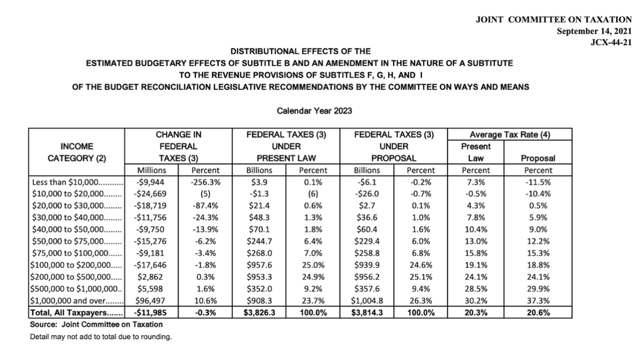
Distribution tables start with a sample of federal income tax returns that are typically supplemented with Census Bureau data to account for individuals who do not file a tax return. Once the universe of taxpayers is defined, additional sources of income are added to provide a broader measure of total income. Such additions include employer-provided benefits like pensions and health insurance; the employer’s share of the Social Security and Medicare payroll tax; as well as corporate income taxes, which are discussed in more detail below.
Distribution tables are generally limited to federal taxes, including individual and corporate income taxes, payroll taxes, excise taxes, custom duties, and the estate and gift tax. Efforts to include state and local taxes are still a work in progress.[2]
Distribution tables typically reflect how individuals respond to changes in tax policy such as the timing of transactions (realization of capital gains); shifts between business sectors (corporate to non-corporate); or changes in employee compensation (wages to fringe-benefits). These behavioral responses affect the composition of income, but not the total amount of income, which is assumed to remain constant. Some organizations incorporate economic growth effects into their distribution tables, thereby allowing total income to vary.
What’s Wrong with Distribution Tables?
The federal individual income tax system is highly progressive. On average, lower-income individuals pay less in taxes, and higher-income individuals pay more in taxes, when measured as a percentage of income. However, there is substantial variation around the average within each income category. This variation reflects differences in filing status (single, head-of-household, married jointly or separately); itemized or standard deduction; number and age of dependent children; and types of income (wages, interest, dividends, capital gains) which may be taxed at different rates, or not all (tax-exempt bonds).
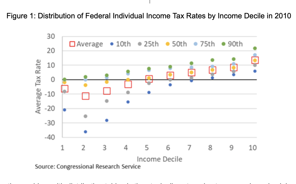
The Congressional Research Service (CRS) analyzed a representative sample of federal individual income tax returns from 2010.[3] This analysis shows how much average tax rates vary within each income category. Among taxpayers in the second lowest decile, Figure 1 shows tax rates range from positive 2 percent (green dot) to negative 36 percent (dark blue dot), with an overall average of negative 11 percent (red square). When distribution tables only provide the average tax rate for each income category, rather than the range of tax rates within each income category, the result is an incomplete and potentially misleading picture, especially at lower-income levels.
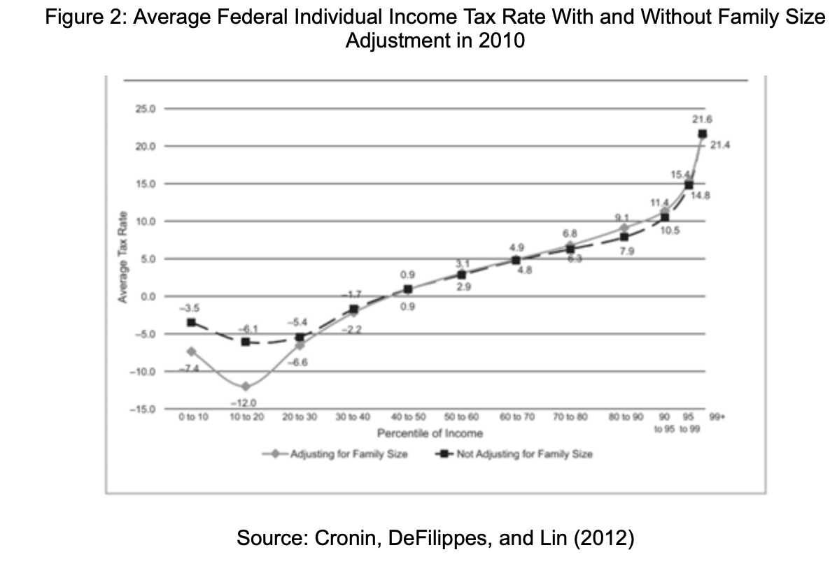
Another problem with distribution tables is they typically categorize taxpayers based solely on income, regardless of family size. A progressive income tax system is based on the premise that taxpayers with more income should pay more taxes. But this premise overlooks the fact that taxpayers with the same income, but different family size, do not have the same ability to pay taxes. The tax code makes some adjustments for family size, such as the number of personal exemptions or child tax credits, and different standard deductions and tax brackets for each filing status, but it does not explicitly consider the economies of scale associated with different family sizes.
In general, people can save money by living together, rather than separately. For example, a two-bedroom apartment does not cost twice as much as a one-bedroom apartment. When distribution tables categorize taxpayers solely by income, regardless of family size, they ignore the differences in living expenses that affect the ability to pay taxes. A recent study categorized taxpayers into income deciles using an “equivalency scale” (family income divided by square root of family size) to better approximate their ability to pay taxes. The study shows average tax rates decrease for lower-income taxpayers and increase for higher-income taxpayers, compared to when taxpayers are categorized based solely on income without regard to family size.[4]
Unlike individual income taxes which are reported directly on individual tax returns, accounting for the distributional effects of corporate income taxes is more problematic. One approach is to assume corporate taxes represent income that individuals would have received in the absence of the tax. At a minimum, corporate taxes reduce the funds available to pay wages to workers or dividends to investors. Alternatively, corporate taxes reduce investment and output, resulting in less income for both workers and investors. To reflect these assumptions, corporate taxes are added to individual income based on the amount of labor and capital income reported on individual income tax returns. Thus, individuals are assumed to pay corporate taxes in proportion to their share of applicable income.
Various theories suggest the allocation of corporate taxes between labor and capital income could range from 0 to 100 percent in either direction, depending on how responsive investors are to changes in the after-tax return to capital; the mobility of capital between corporate and non-corporate businesses; the openness of the economy to international trade and investment; and the rate of substitution between capital and labor. The consensus among most organizations is that the labor share of the corporate tax is 20 to 25 percent and the capital share of the corporate tax is 75 to 80 percent.[5]
But this consensus ignores the fact that the economic burden (a.k.a. “deadweight loss”) of the corporate income tax exceeds the amount of revenue collected. Taxes affect the economy by changing the after-tax return to labor and capital, thereby affecting employment and investment, which determine income and output. Simply adding corporate taxes to individual income understates the loss attributable to the tax. A simple economic model shows labor and capital lose more than $1 in income for every $1 of taxes collected by the government (See Appendix 1).
Distribution tables are sometimes called “dynamic” because they assume taxpayers change their behavior in response to changes in taxes. But these tables are still “static” because they assume changes in taxpayer behavior cannot change aggregate income and output. The implausible assumptions needed to justify this “dynamically-static” view of the economy are readily apparent in the case of excise taxes.
Distribution tables typically assume when an excise tax is imposed on an item, such as alcohol or tobacco, there is a reduction in demand for that item which results in an offsetting reduction in other taxes equal to 25 percent of the excise tax revenue.[6] This offset reflects the assumption that excise taxes are either passed forward to consumers in the form of higher prices or backward to producers in the form of lower wages and profits.[7] Assuming the former, when the tax-inclusive price rises, demand falls, causing labor and capital to shift into other sectors of the economy. As the supply of items that are not subject to the excise tax rises, their prices fall, resulting in lower wages and profits which reduces other taxes. The result is a change in relative prices and output between taxed and untaxed items, while aggregate prices and output remain unchanged (See Appendix 2).
The assumption that taxes change relative prices among goods and services and shift production between sectors of the economy without any loss of income and output is considered perfectly reasonable. But the assumption that taxes change relative prices between labor and leisure and saving and consumption — thereby changing income and output — is considered either highly unlikely or too difficult to measure.
What Happens When Temporary Tax Cuts Expire?
In 2017, Congress enacted the Tax Cuts and Jobs Act (TCJA) which reduced marginal tax rates, doubled the standard deduction, and replaced the personal exemption with a $2,000 per child tax credit. These provisions are scheduled to expire at the end of 2025. Earlier this year, Congress enacted the American Rescue Plan Act (ARPA) which expanded the Earned Income Tax Credit for childless workers and increased the child tax credit to $3,600 for children under 6 and $3,000 for children 6 to 17. These provisions are scheduled to expire at the end of 2021, although the President’s Build Back Better Act (BBBA), which Congress is currently considering, would extend them through the end of 2022.
Figure 3 shows the amount of federal individual income taxes in 2021 for three groups of hypothetical taxpayers – single; head of household with one child under age 6; and married with two children under age 6 – who are assumed to have only wage income and claim the standard deduction. Under current law (TCJA and ARPA), the average tax is $15,419. Assuming the TCJA expires, the average tax would increase by $2,385, or 15 percent. Assuming both the TCJA and ARPA expire, the average tax would increase by $4,827 or 31 percent.
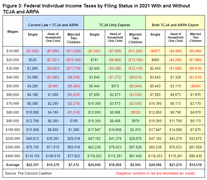
The distributional effects of allowing the TCJA and ARPA provisions to expire will vary depending on taxpayer income, filing status, and the number and age of dependent children. Distribution tables typically obscure this variation by combining dissimilar groups of taxpayers and showing only the average amount of taxes paid for each income category.
The analysis is further complicated by the fact that distribution tables typically compare changes in tax policy to current law. When current law changes due to expiring provisions, the change in tax policy may look very different. For example, it’s important to know whether the $3,600 child tax credit in 2021 is being compared to the $2,000 credit that will expire in 2025, or the previous $1,000 credit that will resume in 2026.
Although the President has stated his desire to make the ARPA provisions permanent, his position on extending the TCJA provisions is unknown. Whether taxpayers will view the failure to extend current tax cuts as a tax increase, and thereby a violation of his campaign promise, is equally unknown.
Conclusion
Distribution tables have featured prominently in tax policy debates in recent decades because they appear to answer an important question, who pays taxes and how much do they pay? Unfortunately, appearances can be deceiving. Distribution tables rely on numerous assumptions and imputations that are not sufficiently transparent to policymakers and the public. They also fail to provide adequate detail on the variation of taxes within each income category. Moreover, by ignoring economic growth effects, distribution tables fail to acknowledge that changes in tax policy can affect how much income is earned, as well as how much revenue is collected.
Government agencies and public policy research organizations have made progress in recent years with the development of more fully dynamic economic growth models. But they have yet to develop a consensus model or a uniform approach to incorporating economic growth effects into distributional analysis. More work remains to be done. In the meantime, policymakers will continue to rely on existing distribution tables, despite their obvious limitations. Although distribution tables can provide useful information on the general direction of tax policy changes, in many cases, taxpayers won’t know how they will be affected until they file their tax return.
Appendix 1
Distribution tables typically assume corporate income taxes are paid by the factors of production (labor and capital) in some proportion to their wages and profits. These proportions vary based on alternative theories. However, the fact that taxes change relative prices between labor and leisure, and saving and consumption — thereby changing income and output — is typically ignored because there is no consensus on the size of this effect.
Historical data suggest the relationship between inputs and outputs in the economy can be represented by a mathematical formula known as the Cobb-Douglas production function. This formula states that Y=A*L^(a)*K^(1-a), where:
Y = output of goods and services
A = total factor productivity
L = labor (hours worked)
K = capital (land, buildings, equipment, and inventory)
(a) = labor income share
(1-a) = capital income share
Holding the current state of technology (A) constant, economic output (Y) is determined by the input of labor (L) and capital (K); and these two factors are each paid for their marginal product, (a) and (1-a), respectively. The marginal product is the additional output produced by the additional input.
The decision to undertake additional investment depends on whether the additional income from the marginal product of capital will cover the additional costs. These costs include economic depreciation, due to wear and tear or technological obsolescence; taxes on business owners and investors; and a “normal” rate of return. The normal return is the amount owners and investors expect to receive in the future to forgo an equivalent amount of current consumption. This return reflects the time-value of money or society’s rate of time-preference.
Taxes increase the cost of capital and decrease the rate of return to owners and investors, resulting in less investment. Using the Cobb-Douglas formula, a one percent increase in the cost of capital will result in a one percent decrease in the capital/output ratio. In theory, businesses and investors will forgo the least profitable investments until the capital stock shrinks enough to restore a normal after-tax rate of return. Thus, taxes on capital do not reduce the after-tax rate of return; instead, they reduce the amount of capital. This result is often criticized as being too extreme, but it provides a useful upper-bound estimate.
To reflect a broader range of potential results, Appendix Table 1 assumes the change in investment with respect to the after-tax return on capital ranges from 0.0 to 1.0. Because the after-tax return is only a fraction of the total cost of capital, these results are proportionally smaller than the standard Cobb-Douglas results. Even under these modest assumptions, labor and capital always lose more than $1 in after-tax income for every $1 of corporate taxes collected by the government, unless it is unrealistically assumed that corporate taxes have absolutely no effect on investment (elasticity = 0.0).
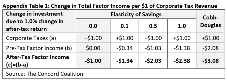
This analysis is based on the Cobb-Douglas formula calibrated to BEA data for the domestic corporate business sector in 2019.[8] The baseline scenario assumes the corporate income tax rate is 25 percent (21% federal plus 4% state) with 100 percent expensing of new investment.[9] The alternative scenarios assume the corporate income tax rate is 10 percent higher (27.5%).
Appendix 2
Distribution tables typically assume excise taxes are paid by consumers in proportion to their consumption and their consumption changes in response to higher tax-inclusive prices. However, to maintain the static assumption that aggregate income and output remain unchanged, there must be equal and offsetting changes in prices and output elsewhere in the economy.
Appendix Table 2 shows a hypothetical two-sector (A and B) economy before and after the imposition of a 10 percent excise tax in only one sector (A). To maintain constant prices without changing total output, prices rise in sector A by the amount of the tax and demand falls by an offsetting amount, while the corresponding share of labor and capital employed in sector A moves to sector B, where prices fall reducing wages and profits, resulting in less income taxes.[10]
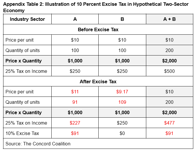
The revenue estimate would reflect higher excise taxes ($91) and lower income taxes ($500 – $91 x 25% = $477). The distribution table would show higher excise taxes ($91) based on individual consumption patterns and lower labor and capital income ($91) based on some proportion of their contribution to total income.
[1] Revenue Estimating | Joint Committee on Taxation (jct.gov); Distribution of Federal Taxes | Congressional Budget Office (cbo.gov); Office of Tax Analysis | U.S. Department of the Treasury; Tax Model Resources | Tax Policy Center; Taxes and Growth Model Overview and Methodology | Tax Foundation; Tax Module — Penn Wharton Budget Model (upenn.edu) See also Tax-Calculator — Tax-Calculator (pslmodels.org); TAXSIM Related Files at the NBER; The Effect of Different Tax Calculators on the SPM (census.gov); ITEP Microsimulation Tax Model Overview – ITEP
[2] Allocating State and Local Taxes to U.S. Households (cbo.gov)
[5] IF10742 (congress.gov); Labor Bears Much of the Cost of the Corporate Tax | Tax Foundation
[6] The Role of the 25 Percent Revenue Offset in Estimating the Budgetary Effects of Proposed Legislation (cbo.gov); JCX-59-11 | Joint Committee on Taxation (jct.gov); The weighted average marginal tax rate on labor and capital income is roughly 25 percent.
[7] If excise taxes are passed backwards to producers, then the reduction in wages and profits would occur in the sector of the economy subject to the excise tax, rather than the untaxed sectors as described above.
[8] GVA Domestic Corporate Business (BEA) (Table 1.14); Fixed Assets by Type (BEA) (Table 6.1)
[9] State Corporate Income Tax Rates and Brackets | Tax Foundation
[10] OTA Paper 85 – U.S. Treasury Distributional Analysis Methodology – September 1999
Continue Reading


